Published on January 5, 2022

reinforcement learningmath

Introduction to Concepts in Reinforcement Learning

Aditya Chopra

@adeecc11

Introduction to Concepts in Reinforcement Learning

What even is Reinforcement Learning?

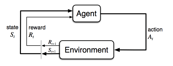
The goal of Reinforcement Learning is simple: an 'agent' learns to maximise the 'rewards' it earns, by interacting with an 'environment'. Let's break down all these terms one by one. Imagine a game of tic-tac-toe with your friend. You start with an empty 3x3 grid. You begin by placing an X in an empty position, followed by your friend placing an O in another. This goes on until one of you owns a row, column or a major diagonal. Now imagine instead of your friend a computer plays against you. Can we make the computer play as good as you do? This is the problem reinforcement learning tries to solve: making a 'machine' learn to work in an environment and thereafter maximise its performance.

Defining some Terms

The game you are playing is the environment. It has a fixed set of rules for how you interact with it and how a winner is decided. The board is like state of the environment, or just the state. Every action a player takes, occupies another cell in it, modifying the state at each turn. An agent is a player in the game, like you or your friend. It takes some actions that have some consequence and the game continues. These consequences are two fold: it modifies the state of the environment and may or may not lead to a reward. One of you winning the game, can be considered a reward. The sequence of steps, from the start of the game to the end is an episode.

Formal Definitions

An agent acts in an environment. The state $s$ belongs to the state space $s \in \mathcal{S}$ and the agent may choose any action $a \in \mathcal{A}(s)$ where $\mathcal{A}(s)$ is the action space corresponding to the current state $s$ . The next state, $s'$ the agent arrives in and the reward, $r \in \mathcal{R}$ for the action are determined by the transition probability distribution $P(s', r | s, a)$ , or simply the transition function.

An episode is defined as the sequence of steps from the initial state to a terminal state:

S_0, A_0, S_1, A_1, ..., S_{T-1}, A_{T-1}, S_T

The Markov Assumption and the Markov Decision Process

This particular form of the transition function that we saw earlier is centered around the assumption that the next state and reward depend only on the current state and action. This is known as the Markov Assumption. Loosely,

P(S_{t+1} | S_1, S_2, ..., S_t) = P(S_{t+1} | S_t)

A full definition of the Markov Assumption in our case requires including the action terms as well, but this conveys the spirit of the notion just as well.

The Markov Decision Process

Finally, we can frame our reinforcement learning problem as a Markov Decision Process (MDP) which encapsulates all the information we have about our environment.

An MDP is a 4-tuple, $\mathcal{M} = (\mathcal{S}, \mathcal{A}, \mathcal{R}, P)$ where,

$\mathcal{S}$ is the state space
$\mathcal{A}$ is the action space
$\mathcal{R}$ is the reward space.
$P$ is the transition function.

How Good Actually is a State or an Action

For the agent to be able to learn, it might need to evaluate how good a state is to be there, or how good aan action is to take. To tackle this we introduce three new quantities: Return $G_t$ , State-Value Function $v(s)$ and the Action-Value function $q(s, a)$ .

Return is simply the total value of the reward going forward from the current timestep.

G_t = R_{t + 1} + R_{t + 2} + ... = \sum_{k=0}^{\infty} R_{t+k+1}

However, if an episode never ends (for example in the case of balancing a pole on a moving cart, or our supply chain management problem even), $G_t$ might blow up to positive or negative Infinities. Further, we might wanna weight rewards that we might get say 3 steps down the line more than those we get 100 steps down the line. To solve all these problems, we introduce a discounting factor $\gamma$ when calculating the Return.

G_t = R_{t + 1} + \gamma R_{t + 2} + \gamma^2 R_{t + 3} ... = \sum_{k=0}^{\infty} \gamma^k R_{t+k+1}

We can simplify the above expression into a recurrence relation as follows:

\begin{align*} G_t &= R_{t + 1} + \gamma R_{t + 2} + \gamma^2 R_{t + 3} ... \\ &= R_{t + 1} + \gamma ( R_{t + 2} + \gamma R_{t + 3} + \gamma^2 R_{t + 4} ... ) \\ &= R_{t + 1} + \gamma G_{t+1} \end{align*}

This form of the equation is used extensively when deriving other equations for RL.

The state-value function is just the expected return from the current state $s$ . That is, if at timestep t we are at state $s$ ,

v(s) = \mathbb{E}[G_t | S_t = s]

Similarly, the action-value function of a state-action pair is the expected return on taking the action at the state.

q(s, a) = \mathbb{E}[G_t | S_t = s, A_t = a]

The Policy

The Policy of an agent is the set of probabilities it assigns every state-action pairs. That is, it defines the probability of taking a certain action at any given state.

\pi(a | s) = P(A = a | S = s)

Notice that this equation does not have a timestep subscript. This implies that the probability of an action is independent of how many steps have been taken so far, and depends only on the current state, $s$ .

The policy of a deterministic agent is essentially the action it takes at any given state (with a probability of $1$ ). Consequently, for a deterministic agent we might write the policy as follows:

\pi(s) = a

We can now re-contextualize the definitions for state and action value functions to include the policy parameters as follows:

v_{\pi}(s) = \mathbb{E}_{\pi}[G_t | S_t = s] \\ q_{\pi}(s, a) = \mathbb{E}_{\pi}[G_t | S_t = s, A_t = a]

where the subscript just denotes that we are following the policy $\pi$ when doing our calculations.

Policies derived from value functions

If we don't use the generated value functions to determine which actions to take in a state, then what even was the point of generating them. Exactly with this thought we introduce greedy and $\epsilon$ -greedy policies.

A greedy policy is one, which at every state, chooses only the action with the highest action-value estimate, i.e. it is a deterministic policy. Quantitatively, a greedy policy is defined as

\pi_{greedy} (s) = \argmax_a q(s, a)

On the other hand, we can have a stochastic policy that almost always chooses the greedy action, but sometimes with a very small probability, chooses an action randomly. Such policies are called $\epsilon$ -greedy. Mathematically,

\pi(a | s) = \begin{cases} 1 - \epsilon + \frac{\epsilon}{| \mathcal{A(s)} |} & a = \argmax_{a'} q(s, a') \\ \frac{\epsilon}{| \mathcal{A(s)} |} & \text{otherwise} \end{cases}

The choice of values for $\epsilon$ leads into the exploration-exploitation problem which is whole another can of worms.

Estimating this Goodness

With all this background we can finally get to actually estimating these values in a practical sense.

Observation 1

Since we are following the policy $\pi$ we can estimate the state and action value functions in terms of each other.

v_{\pi}(s) = \sum_{a \in \mathcal{A}(s)} \pi(a | s) \cdot q(s, a)

So, given the action-values, we can convert it to the required state-values.

Observation 2

We can expand out our equations to get a better sense of what is actually going on.

\begin{align*} q_{\pi}(s, a) &= \mathbb{E}_{\pi}[G_t | S_t = s, A_t = a] \\ &= \mathbb{E}_{\pi}[R_{t+1} + \gamma G_{t+1} | S_t = s, A_t = a] \\ &= \sum_{s'} \sum_{r} p(s', r | s, a)(r + \gamma \mathbb{E}_{\pi}[G_{t + 1} | S_{t + 1} = s'] ) \\ &= \sum_{s', r} p(s', r | s, a)(r + \gamma v_{\pi} (s')) \end{align*}

The last equation is derived by accounting for all the states, $s'$ that can occur and rewards $r$ we can gain after taking that action on taking that action $a$ . In essence, we compute the probability of both the variables: $s', r$ occurring and use them to weight the return generated by it.

The final equation we have derived is the Bellman Equation for $q_\pi$ . It gives a quantitative relation between the current action-values and the subsequent state-values. We are looking ahead from the current state, to the next (and by extension all future) state(s) to determine the current value estimates.

This opens the door to various methods of estimating the value functions, by varying how wide or how deep we choose to look.

Evaluation, Estimation and Control

The "Holy Grail" of Policies

The goal of reinforcement learning is to reach an optimal policy. Loosely, an optimal policy is one that is able to generate a lot of reward over the long run. We denote an optimal policy as $\pi_*$

There may be more than one optimal policies, that achieve our goals.

All optimal policies share the same state and action value functions and are unsurprisingly called the optimal state-value function, $v_*(s)$ and the optimal action-value function, $q_*(s, a)$ .

We define these optimal functions as follows:

\begin{align*} \pi &= \pi_* \implies \pi_* \ge \pi, & \forall \pi:\mathbb{R}^2 \rightarrow [0, 1] \\ q_*(s, a) &= \max_\pi q_\pi(s, a), & \forall s \in \mathcal{s}, a \in \mathcal{A}(s) \\ v_*(s) &= \max_\pi v_\pi(s), & \forall s \in \mathcal{s} \end{align*}

$\pi > \pi' \iff v*\pi(s) \ge v*{\pi'}, \quad \forall s \in \mathcal{S}$

The Bellman Optimality Equations

Intuitively, If we are only interested in the optimal values, rather than computing the expectation following a policy, we could jump right into the maximum returns during the alternative updates without using a policy in the equation derived in Observation 1.

\begin{align*} v_*(s) &= \max_{a \in \mathcal{A}(s)} q_{\pi_*} (s, a) \\ &= \max_a \sum_{s', r} p(s', r | s, a)(r + \gamma v_* (s')) \end{align*}

We use Observation 2 on the last line.

Similarly, we could proceed for the action value function to get:

q_*(s, a) = \sum_{s', r} p(s', r | s, a)(r + \gamma \max_{a'} q_* (s', a'))

These are collectively called the Bellman Optimality Equations.

If we had complete knowledge of the MDP, especially the transition function then we could solve the Bellman Optimality Equations to get an optimal policy for our agent. However, rarely are these information privy to us. We use these only to lay a theoretical foundation for all the subsequent RL algorithms such as Dynamic Programming (DP), Monte-Carlo (MC) Methods or Temporal Difference (TD) Learning.

In this post I look only at TD Learning and will casually ignore DP and MC Methods. Do not at me.

Temporal Difference Learning

Temporal Difference Learning is used to update targets, or our estimates of state or action value estimates as our agent interacts with the environment in an episode. TD Learning does not require episodes to run to completion before updating the estimates (unlike some un-named algorithms).

This accomplished by updating targets with our estimates themselves. This is known as bootstrapping.

TD Learning can be used to either just estimate the state (or action) value functions based on a certain policy, or it can be used to simultaneously learn an optimal policy as well. The former is knows an Value Estimation and the latter Control.

Value Estimation

Before we proceed, we need to determine a target for the TD Methods to estimate. We start by looking at the definition of the state-value function.

\begin{align*} v_\pi(s) &= \mathbb{E}[G_t | S_t = s] \\ &= \mathbb{E}[R_{t + 1} + \gamma G_{t + 1} | S_t = s] \\ &= \mathbb{E}[R_{t + 1} + \gamma v_\pi(S_{t + 1}) | S_t = s] \end{align*}

Temporal Difference Learning utilizes the last equation with 2 variations:

The exact value of $v_\pi(S_{t + 1})$ is not known, and is instead replaced by our current estimate, $V$ .
The expected value is not known, and we directly use the sampled value as an approximation of the expected value

We differentiate estimates from true values by using lowercase alphabet for the true values, and uppercase for our estimates. This convention is typically followed in literature as well.

Putting it together, the target for our estimated return is

R_{t + 1} + \gamma V(S_{t + 1})

This gives us the simple update equation:

V(S_t) \leftarrow V(S_t) + \alpha [ R_{t+1} + \gamma V(S_{t+1}) - V(S_t)]

where $\alpha \in (0, 1]$ can be thought of as a step size, or the learning rate of our algorithm.

Similarly, for estimating action-values we have

Q(S_t, A_t) \leftarrow Q(S_t, A_t) + \alpha [ R_{t+1} + \gamma Q(S_{t+1}, A_{t+1}) - Q(S_t, A_t)]

TD Control

A Learning algorithm can be on or off policy depending on which policy used to generate the episodes and which policy we are updating.

SARSA: On-Policy TD Control

Simply enough, we just go through the episode by taking actions determined by our estimates, and update our estimates with our observations along the way.

Parameters: step size alpha, small epsilon
Initialize: Q(s, a) for all non-terminal s and a.
            Q(terminal, .) = 0

Loop for each episode:
    Initialize S
    Choose A from S using any policy derived from Q (e.g., epsilon-greedy)
    Loop for each step of the episode:
        Take action A, observe R, S'
        Choose A' from S' using the derived policy from Q
        Q(S, A) := Q(S, A) + alpha * [R + gamma * Q(S', A') - Q(S, A)]

        S := S'
        A := A'
    until S is terminal

The fact that we choose the next action according to the same policy as the policy being updated, it is an on-policy algorithm.

The algorithm is called SARSA because we update the Q Values by following the holy sequence: $S_0, A_0, R_1, S_1, A_1, ...$ .

Q-Learning: Off-Policy TD Control

The foundation for years of good things to come, Q-Learning uses a different target from the one obtained by the target policy:

Q(S_t, A_t) \leftarrow Q(S_t, A_t) + \alpha [ R_{t+1} + \gamma max_a Q(S_{t+1}, a) - Q(S_t, A_t)]

Parameters: step size alpha, small epsilon
Initialize: Q(s, a) for all non-terminal s and a.
            Q(terminal, .) = 0

Loop for each episode:
    Initialize S
    Loop for each step of the episode:
        Choose A from S using any policy derived from Q (e.g., epsilon-greedy)
        Take action A, observe R, S'
        Choose A' from S' using the derived policy from Q
        A' := argmax Q(S, a) over a ; Therefore, off policy
        Q(S, A) := Q(S, A) + alpha * [R + gamma * Q(S', A') - Q(S, A)]
        S := S'
    until S is terminal

The key difference between SARSA and Q-Learning comes directly from their respective targets. The target return for SARSA is based on the current policy, whereas for Q-Learning it is based on the optimal policy. Q-Learning estimates $Q*$ directly.

Conclusion and Further Exploration

Q-Learning, and subsequently Deep Q-Learning algorithms such as DQN ushered in a new family of algorithms and made Reinforcement Learning a viable learning method on the large scale. The use of Neural Networks and other function approximators allowed the agents to learn Q-Values for arbitrarily large state and action spaces and even continuous control tasks.

Overtime methods were introduced to skip the middle-man, i.e. the action-value estimates and learn the policy directly. These policy gradient methods, although unstable to train can be combined with Q-Learning models to create actor-critic models that can outperform almost any other reinforcement learning algorithm, and even surpass human level performance and more agents and algorithms being published every day. Hoping to see you at the forefront of it as well!

I know this is a long read, but hopefully it was worth it. If you notice mistakes and errors in this post, don’t hesitate to contact me at [adeecc11 at gmail dot com]. See you in the next post! :)

References

[1]: Sutton, R. S., & Barto, A. G. (2018). Reinforcement learning: An introduction. The MIT Press.
[2]: Silver, D. (2015). Course on Reinforcement Learning.
[3]: Silver, D. (2015). Lectures on Reinforcement Learning [MOOC].
[4]: Hasselt, H. V., Borsa D., & Matteo Hessel (2021) Reinforcement Learning Lecture Series 2021 [MOOC].
[5]: Weng, L. (2018, February 19). A (long) peek into reinforcement learning. Lil'Log.
[6]: Spinning Up by OpenAI (2018): Part 1: Key Concepts in RL